Quickstart
Fit a high-performance model tree on real tabular data in seconds, inspect its transparent decision paths, and evaluate how piecewise linear leaves eliminate step-function distortion.
The complete executable script lives at examples/quickstart.py:
1. Why Model Trees Outperform Standard CART
Standard decision trees (CART) predict a constant mean in each leaf node. On continuous tabular surfaces, this creates rigid staircase artifacts that require excessive depth and overfitting to approximate simple linear trends.
ModelTree(leaf="linear") decouples the tree partition search from leaf estimation. The tree discovers optimal split thresholds while terminal leaves fit regularized linear ridge regressions, capturing local slopes smoothly at shallow depth.
flowchart LR
    A["Raw Feature Vector\n[Cement, Water, Age, ...]"] --> B{"Age <= 14 days?"}
    B -- "Yes (Early Hydration)" --> C{"Cement <= 350 kg/m³?"}
    B -- "No (Matured Matrix)" --> D{"Cement <= 350 kg/m³?"}
    C --> E["Leaf 8: Local Ridge Linear\ny = 0.05*Cement - 0.12*Water + ..."]
    D --> F["Leaf 13: Local Ridge Linear\ny = 0.11*Cement - 0.04*Water + ..."]
    E --> G["Continuous Prediction (MPa)"]
    F --> G

    classDef inputBox fill:#1e293b,stroke:#475569,stroke-width:2px,color:#ffffff;
    classDef splitBox fill:#b45309,stroke:#d97706,stroke-width:2px,color:#ffffff;
    classDef leafBox fill:#065f46,stroke:#059669,stroke-width:2px,color:#ffffff;
    classDef outBox fill:#1e3a5f,stroke:#2563eb,stroke-width:2px,color:#ffffff;

    class A inputBox;
    class B,C,D splitBox;
    class E,F leafBox;
    class G outBox;
2. Fit and Evaluate on Real Benchmark Data
We evaluate on the industrial benchmark Concrete Compressive Strength (Yeh 19981; 1,030 mixtures, 8 continuous ingredients).
Why Decouple Tree Search from Leaf Estimation?
Evaluating multivariate linear models at every candidate split threshold incurs massive combinatorial overhead. ModelTree uses fast variance or structural break heuristics to discover partition boundaries, then solves the closed-form regularized ridge system once per terminal leaf node.
Dataset Provenance: Concrete Compressive Strength
Collected by Prof. I-Cheng Yeh (1998) at Chung-Hua University1. Features 1,030 lab mixtures quantifying how 7 cementitious ingredient ratios (cement, slag, fly ash, water, superplasticizer, coarse aggregate, fine aggregate) and curing age interact nonlinearly to determine compressive yield stress (MPa).
from mltreelib import Metrics, ModelTree, load_dataset

# 1. Load benchmark dataset (1,030 mixtures, 8 features)
data = load_dataset("concrete_compressive_strength")
target = "ConcreteCompressiveStrength"
feature_names = [col for col in data["columns"].keys() if col != target]
n_rows = data["n_rows"]

X = [[data["columns"][c][i] for c in feature_names] for i in range(n_rows)]
y = data["columns"][target]

# 80/20 train/test split
split_idx = int(n_rows * 0.8)
X_train, y_train = X[:split_idx], y[:split_idx]
X_test, y_test = X[split_idx:], y[split_idx:]

# Fit mltreelib ModelTree (piecewise linear ridge leaves, depth=3)
model_tree = ModelTree(leaf="linear", max_depth=3, min_rows=20, l2=1e-3)
model_tree.fit(X_train, y_train, col_names=feature_names)
pred_mt = model_tree.predict(X_test)

# Measure holdout metrics
metrics = Metrics()
m_mt = metrics.regression(y_test, pred_mt)
print(f"ModelTree (Linear): RMSE = {m_mt['rmse']:.2f} MPa, R2 = {m_mt['r2']:.3f}, MAE = {m_mt['mae']:.2f} MPa")
from mltreelib import Metrics, ModelTree, load_dataset

data = load_dataset("concrete_compressive_strength")
target = "ConcreteCompressiveStrength"
feature_names = [col for col in data["columns"].keys() if col != target]
n_rows = data["n_rows"]

X = [[data["columns"][c][i] for c in feature_names] for i in range(n_rows)]
y = data["columns"][target]

split_idx = int(n_rows * 0.8)
X_train, y_train = X[:split_idx], y[:split_idx]
X_test, y_test = X[split_idx:], y[split_idx:]

# Fit standard CART decision tree (constant mean leaves, depth=3)
cart = ModelTree(leaf="mean", max_depth=3, min_rows=20)
cart.fit(X_train, y_train, col_names=feature_names)
pred_cart = cart.predict(X_test)

metrics = Metrics()
m_cart = metrics.regression(y_test, pred_cart)
print(f"CART (Mean)       : RMSE = {m_cart['rmse']:.2f} MPa, R2 = {m_cart['r2']:.3f}, MAE = {m_cart['mae']:.2f} MPa")
3. Empirical Results & Performance Comparison
Loaded Concrete Compressive Strength: 1030 rows, 8 features.
Train rows: 824, Test rows: 206

=== Model Performance on Test Set ===
Standard Decision Tree (CART)  : RMSE = 11.09 MPa, R2 = 0.566, MAE = 8.47 MPa
mltreelib ModelTree (Linear)   : RMSE = 7.28 MPa, R2 = 0.813, MAE = 5.07 MPa
--> Error reduction with linear leaves: 34.3%
| Model | Leaf Formulation | Depth | Test RMSE (MPa) | Test \(R^2\) | Test MAE (MPa) |
|---|---|---|---|---|---|
| Standard CART | Constant Mean | 3 | 11.09 | 0.566 | 8.47 |
mltreelib ModelTree |
Regularized Linear Ridge | 3 | 7.28 | 0.813 | 5.07 |
With identical tree topology (depth 3, 8 leaves), ModelTree achieves a 34.3% error reduction and increases explained variance from 56.6% to 81.3%.
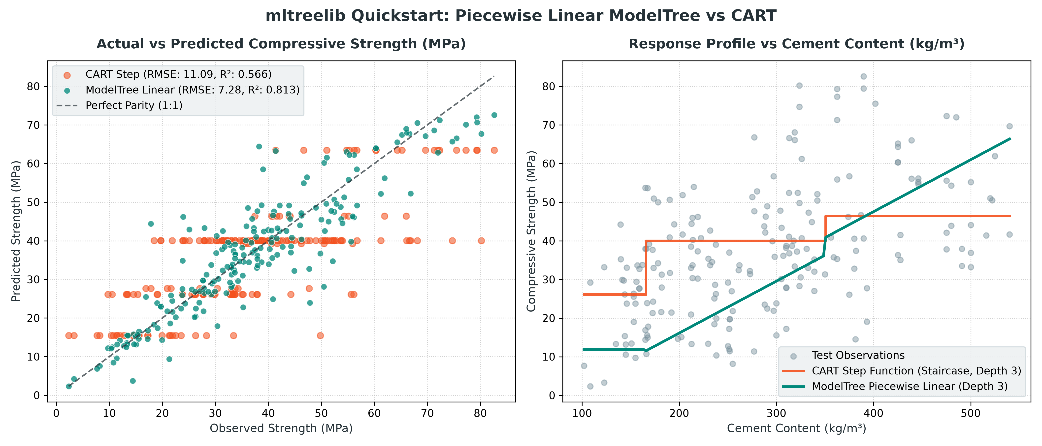
- Left Panel (Parity Plot): Predictions from
ModelTree(leaf="linear")cluster tightly along the 1:1 diagonal, whereas CART's predictions are constrained to horizontal bands corresponding to leaf means. - Right Panel (Response Profile): Along the gradient of Cement content, CART produces wide step discontinuities, while
ModelTreepreserves the physical continuous response curve.
4. Transparent Tree Structure & Inspection
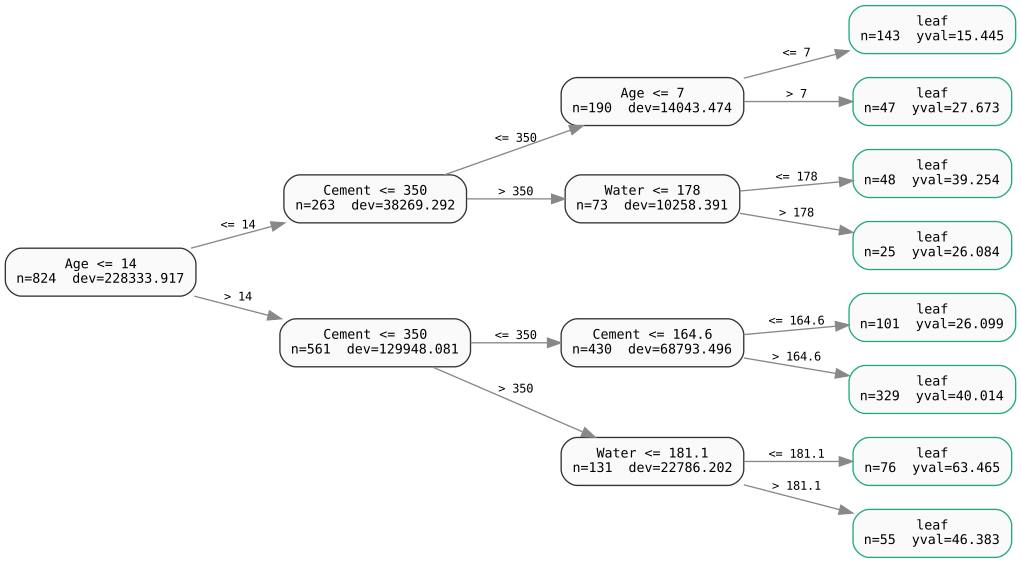
ModelTree prints in rpart-compatible notation with exact node numbering, split criteria, sample support, deviance, and fitted constants:
n= 824

node), split, n, deviance, yval
      * denotes terminal node

 1) root 824 228333.917 35.46173
   2) Age <= 14 263 38269.292 22.98684
     4) Cement <= 350 190 14043.474 18.46968
       8) Age <= 7 143 6493.479 15.44493 *
       9) Age > 7 47 2261.042 27.67263 *
     5) Cement > 350 73 10258.391 34.74381
      10) Water <= 178 48 5059.180 39.25437 *
      11) Water > 178 25 2347.636 26.08354 *
   3) Age > 14 561 129948.081 41.31003
     6) Cement <= 350 430 68793.496 36.74539
      12) Cement <= 164.6 101 8521.781 26.09900 *
      13) Cement > 164.6 329 45309.403 40.01374 *
     7) Cement > 350 131 22786.202 56.29321
      14) Water <= 181.1 76 6496.752 63.46522 *
      15) Water > 181.1 55 6978.299 46.38280 *
Export directly to Graphviz DOT for vector diagrams:
Next Steps
- Explore the Practical Modeling Pathways for end-to-end classification, survival, and uplift workflows.
- Study Dynamic Leaf Retraining for microsecond warm-start leaf adaptation.
- Review Distributional Leaves for Tobit, Tweedie, and Gamma modeling.
- Inspect the API Reference for all parameters and methods.
References
-
Yeh, I-C. (1998). "Modeling of strength of high-performance concrete using artificial neural networks." Cement and Concrete Research, 28(12), 1797-1808. ↩↩
-
Quinlan, J. R. (1992). "Learning with continuous classes." 5th Australian Joint Conference on Artificial Intelligence, 343-348. ↩
-
Chow, G. C. (1960). "Tests of equality between sets of coefficients in two linear regressions." Econometrica, 28(3), 591-605. ↩