Survival trees in Python: FLCHAIN mortality follow-up
Use baseline measurements to estimate survival at one, three and five years. The event is death. If follow-up ends first, the row is right-censored.
1. Get the data and define the evaluation
The survival package's FLCHAIN cohort contains 7,874 people and right-censored follow-up. futime is follow-up in days and death=1 records a death. We use age, sex, kappa, lambda and creatinine as predictors. We exclude chapter, which describes cause of death and is unavailable at prediction time. Creatinine is missing for 952 of the 5,500 training records and 398 of the 2,374 test records; values enter the tree without imputation.
Download FLCHAIN CSV from Rdatasets to datasets/external/real_eval/flchain.csv. The checked file SHA-256 is a96bcc58addb4c127e5012c5974aec8c7daf66123ddb104f309a78f158daa563. Run the shared real-data evaluation script.
2. Fit leaf survival curves
futime is the time to death or last observation. Keep the event flag next to it. For example, someone censored at day 600 survived beyond day 365, but their status at day 1,095 is unknown. Do not replace the censored outcome with an event at day 600.
flowchart TD
    subgraph TimeToEvent["Right-Censored Follow-up Mechanics (T_i, delta_i)"]
        direction LR
        Patient["Patient Baseline\n(Age, Biomarkers)"] --> FollowUp["Follow-up Period\n[0, T_i]"]
        FollowUp --> Event{"Did Event Occur Before\nEnd of Study / Dropout?"}
        Event -- "Yes (Event Observed)" --> Dead["delta_i = 1\nExact Event Time T_i"]
        Event -- "No (Right-Censored)" --> Censored["delta_i = 0\nT_i is Lower Bound (T* > T_i)"]
    end
    Dead & Censored --> LogRank["Log-Rank / Martingale Split Criterion\nmax Q_LR(s)"]
    LogRank --> KM["Terminal Leaf Estimators\nKaplan-Meier S(t) & Nelson-Aalen H(t)"]

    classDef dataBox fill:#1e293b,stroke:#475569,stroke-width:2px,color:#ffffff;
    classDef gateBox fill:#b45309,stroke:#d97706,stroke-width:2px,color:#ffffff;
    classDef deadBox fill:#881337,stroke:#9f1239,stroke-width:2px,color:#ffffff;
    classDef censBox fill:#1e3a5f,stroke:#2b4c7e,stroke-width:2px,color:#ffffff;
    classDef splitBox fill:#0369a1,stroke:#0284c7,stroke-width:2px,color:#ffffff;
    classDef leafBox fill:#065f46,stroke:#059669,stroke-width:2px,color:#ffffff;

    class Patient,FollowUp dataBox;
    class Event gateBox;
    class Dead deadBox;
    class Censored censBox;
    class LogRank splitBox;
    class KM leafBox;
Run this Python block from the repository root. The evaluation helpers are part of the example script.
from random import Random

import pandas as pd
from mltreelib import ModelTree
from examples.real_survival_uplift import brier, censor_km

df = pd.read_csv("datasets/external/real_eval/flchain.csv")
features = ["age", "sex", "kappa", "lambda", "creatinine"]
types = ["numeric", "categorical", "numeric", "numeric", "numeric"]
ids = list(range(len(df)))
Random(2026).shuffle(ids)

def inputs(indices):
    part = df.iloc[indices]
    x = [[None if pd.isna(v) else v for v in row]
         for row in part[features].itertuples(index=False, name=None)]
    return x, part.futime.astype(float).tolist(), part.death.astype(float).tolist()

x_train, t_train, e_train = inputs(ids[:5500])
x_test, t_test, e_test = inputs(ids[5500:])
grid = [365.0, 1095.0, 1825.0]
censor = censor_km(t_train, e_train)

for depth in (0, 2):
    tree = ModelTree(leaf_family="survival", max_depth=depth,
                     min_rows=100, prune="none")
    tree.fit(x_train, (t_train, e_train), col_names=features, dtypes=types)
    curves = tree.predict(x_test, kind="survival", times=grid)
    print("depth", depth, "first survival curve", curves[0])
    for j, horizon in enumerate(grid):
        print(horizon, brier(t_test, e_test, [curve[j] for curve in curves],
                             horizon, censor))
    print(tree.splits()[:1])
The depth-zero tree estimates one Kaplan–Meier curve for everyone. The deeper tree assigns a separate curve to each leaf. Inspect early and late horizons separately because each has a different set of known outcomes.
3. Interpret the held-out results
| Horizon, days | Test at risk | Censoring survival, training estimate | Tree IPCW Brier | Global baseline |
|---|---|---|---|---|
| 365 | 2,270 | 0.9930 | 0.0329 | 0.0343 |
| 1,095 | 2,144 | 0.9834 | 0.0671 | 0.0731 |
| 1,825 | 2,043 | 0.9737 | 0.0884 | 0.1026 |
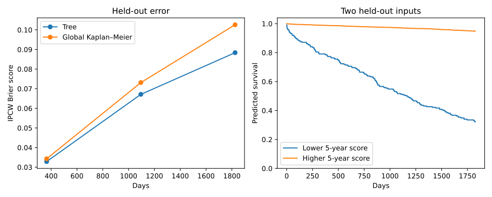
The right panel shows two held-out feature rows routed through the training tree. They were selected by their predicted five-year survival, without using their outcomes. Their five-year predictions are 0.321 and 0.948. These are leaf estimates. The left panel measures error across all 2,374 test rows, which include 644 recorded deaths and 1,730 censored observations over the available follow-up.
The example uses a seeded random split and estimates the marginal censoring distribution from training data only. A marginal censoring model assumes censoring is independent of the outcome in the relevant population. This observational cohort and one split do not establish clinical usefulness. Check conditional censoring, calibration, discrimination and uncertainty with the intended deployment population before interpreting the comparison.
4. Controlled check with synthetic truth
The survival and uplift evaluation script simulates 5,000 people. It fits 3,000 and evaluates 2,000 independent records, including 1,391 observed events and 609 censored observations. A global survival model provides the baseline.
| Horizon | Tree IPCW Brier | Global baseline IPCW Brier |
|---|---|---|
| 10 | 0.2417 | 0.2509 |
| 20 | 0.2000 | 0.2102 |
| 30 | 0.1226 | 0.1316 |
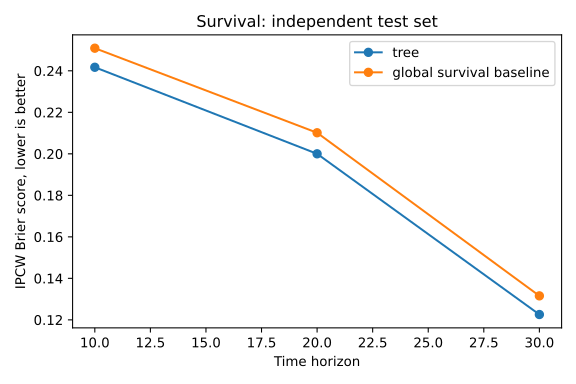
The Brier score compares predicted survival probabilities with event outcomes at a fixed horizon. Inverse probability of censoring weights (IPCW) account for records censored before that horizon. Lower is better. This simulation uses the known censoring distribution. Real data requires a justified censoring model estimated without using the test outcomes for model selection, adequate follow-up, and positive censoring survival at each evaluated horizon. Conditional censoring requires appropriate conditional weights; a single global curve can be wrong.
The script also compares predictions with the known synthetic survival probability. Real individual survival probabilities are not observed. Check discrimination and horizon-specific calibration on real held-out data, with uncertainty and risk-set sizes. This example implements the evaluation calculation locally; it does not claim an IPCW metric API exists in the package. See Graf et al. (1999).
5. Competing risks and multi-cause endpoints
When subjects can experience mutually exclusive event causes (e.g. disease relapse vs treatment-related mortality), treating competing events as ordinary censoring violates the independent censoring assumption and overestimates cumulative incidence by 20–50%.
mltreelib implements native competing risks trees:
- Split Criterion: Gray's subdistribution log-rank test (gain="gray", target_cause=j) maintaining subjects who experienced competing events in the risk set.
- Leaf Estimators: Aalen-Johansen multi-state estimator guaranteeing the probability simplex identity: \(\sum_{c=1}^J \hat{F}_c(t) + \hat{S}(t) = 1.0\).
- Unified Prediction API: tree.predict(X, kind="cif", times=times, cause=1) and tree.predict(X, kind="risk").
- Validation: Metrics().competing_risks(...) computing cause-specific Harrell's C, Uno's IPCW C-index, and time-dependent Brier score matrices.
from mltreelib import ModelTree, Metrics

# Events: 0 = censored, 1 = relapse (primary), 2 = toxicity (competing)
tree = ModelTree(max_depth=3, min_rows=25, gain="gray", target_cause=1)
tree.fit(X_train, (durations_train, events_train))

# Evaluate Aalen-Johansen CIF at specified horizons
times = [2.0, 5.0, 10.0, 20.0]
cif_cause1 = tree.predict(X_test, kind="cif", times=times, cause=1)
cif_cause2 = tree.predict(X_test, kind="cif", times=times, cause=2)
surv = tree.predict(X_test, kind="survival", times=times)

# Compute full IPCW competing risks performance report
metrics = Metrics()
report = metrics.competing_risks(
    durations=durations_test,
    events=events_test,
    cif_curves={1: cif_cause1, 2: cif_cause2},
    times=times,
)
print("Cause 1 Harrell C:", report["cause_c_indices"][1])
print("Cause 1 Uno IPCW C:", report["cause_uno_c_indices"][1])
print("Cause 1 IBS:", report["cause_ibs"][1])
Next steps and references
Survival trees · Kaplan and Meier (1958) · Aalen (1978) · Gray (1988)