Leaf Solver Benchmarks
Benchmark the seven numerical, quasi-Newton, and continuous evolutionary leaf solvers implemented natively in mltreelib-core.
The complete benchmark script lives at examples/solver_benchmarks.py:
1. Architectural Decoupling: Tree Partitions vs. Leaf Solvers
In standard model trees, evaluating complex optimization problems at every candidate split threshold incurs prohibitive computational cost. ModelTree solves this through two-control decoupling:
- Tree Search: Fast scalar heuristics (Variance reduction, Chow test, Log-rank) discover spatial partition boundaries.
- Leaf Optimization: Once terminal regions are established, the configured
leaf_solversolves the local parameter system.
flowchart TD
    Data["Candidate Data in Leaf Node\n[X, y]"] --> Fam{"Is the loss smooth\nand convex?"}

    Fam -- "Yes: Gaussian / Ridge" --> S1["irls (Cholesky / faer)\nExact closed-form solution\nLatency: ~1.2 ms"]
    Fam -- "Yes: Smooth GLM / Tobit" --> S2["lbfgs (Quasi-Newton)\nArmijo line-search\nLatency: ~1.4 ms"]
    Fam -- "L1 Elastic Net Sparsity" --> S3["ccd (Coordinate Descent)\nExact zero-coefficients\nLatency: ~5.3 s"]
    Fam -- "No: Non-Convex / Multi-Modal / Glitchy" --> S4{"Derivative-Free\nEvolutionary Family"}

    S4 --> E1["shade: Adaptive Differential Evolution\nLatency: ~33 ms | Near-optimal"]
    S4 --> E2["cmaes: Covariance Matrix Adaptation\nLatency: ~13 ms | Ill-conditioned"]
    S4 --> E3["ga: Real-Coded Genetic Algorithm\nLatency: ~58 ms | Global exploration"]
    S4 --> E4["nes: Natural Evolution Strategies\nLatency: ~13 ms | Gradient estimation"]

    classDef dataBox fill:#1e293b,stroke:#475569,stroke-width:2px,color:#ffffff;
    classDef gateBox fill:#b45309,stroke:#d97706,stroke-width:2px,color:#ffffff;
    classDef gradBox fill:#065f46,stroke:#059669,stroke-width:2px,color:#ffffff;
    classDef evoBox fill:#4338ca,stroke:#6366f1,stroke-width:2px,color:#ffffff;

    class Data dataBox;
    class Fam,S4 gateBox;
    class S1,S2,S3 gradBox;
    class E1,E2,E3,E4 evoBox;
2. The Seven Solvers in mltreelib-core
Solver (leaf_solver) |
Mathematical Paradigm | Gradient Required? | Primary Strengths | Recommended Setting |
|---|---|---|---|---|
"irls" |
Cholesky / Iteratively Reweighted Least Squares | Yes | Sub-millisecond closed-form solution via faer; exact Gram matrix factorization. |
Default for Gaussian ridge and standard GLM models. |
"lbfgs" |
Quasi-Newton L-BFGS with Armijo line search | Yes | Superlinear convergence on smooth likelihoods (Gaussian, Binomial, Poisson, Gamma, Tobit, Tweedie). | Default for non-Gaussian GLM families and censored regression. |
"ccd" |
Cyclic Coordinate Descent | Yes (Subgradient) | Exact soft-thresholding producing true zero-coefficient sparsity under \(L_1\) penalty. | High-dimensional feature selection and sparse leaves. |
"shade" |
Success-History Adaptive Differential Evolution | No | Continuous mutation scale (\(F\)) and crossover rate (\(CR\)) adaptation with external archive. | Rugged, discontinuous, or multi-modal loss surfaces. |
"cmaes" |
Covariance Matrix Adaptation Evolution Strategy | No | Learns second-order dependency landscape without explicit Hessian inversion. | Ill-conditioned parameter spaces with strong feature correlations. |
"ga" |
Real-Coded Genetic Algorithm | No | Simulated Binary Crossover (SBX) and polynomial mutation across diverse populations. | Broad global exploration of complex parameter bounds. |
"nes" |
Separable Natural Evolution Strategies | No | Monte Carlo natural gradient updates along estimated search directions. | Fast derivative-free parameter tuning in moderate dimensions. |
3. Empirical Benchmark on Real Data
We benchmark all seven solvers on the Yeh (1998) Concrete Compressive Strength dataset (1,030 rows, 8 features; 80% train / 20% test).
Benchmark Results (Standalone Global Fit, max_depth=0)
| Solver | Family | Latency (ms) | Holdout Test RMSE (MPa) | Test \(R^2\) | Convergence Character |
|---|---|---|---|---|---|
irls |
Analytical Cholesky | 1.17 ms | 10.224 | 0.631 | Exact analytical optimum in 1 step. |
lbfgs |
Quasi-Newton | 1.37 ms | 10.224 | 0.631 | Converges in 14 iterations to machine precision. |
shade |
Continuous DE | 33.24 ms | 10.269 | 0.627 | Reaches 99.6% of exact analytical optimum without gradients. |
ga |
Genetic Algorithm | 57.77 ms | 10.360 | 0.621 | Robust global convergence across 100 generations. |
cmaes |
Evolutionary Covariance | 13.23 ms | 11.423 | 0.539 | Fast adaptation; sensitive to raw unstandardized scale. |
nes |
Natural Gradient | 13.13 ms | 16.919 | -0.011 | Fast step updates; requires standardized inputs. |
ccd |
Cyclic Coordinate Descent | 5,720 ms | 10.224 | 0.631 | Exact analytical match; coordinate sweeps on raw scale. |
4. Latency vs. Accuracy Pareto Diagnostic
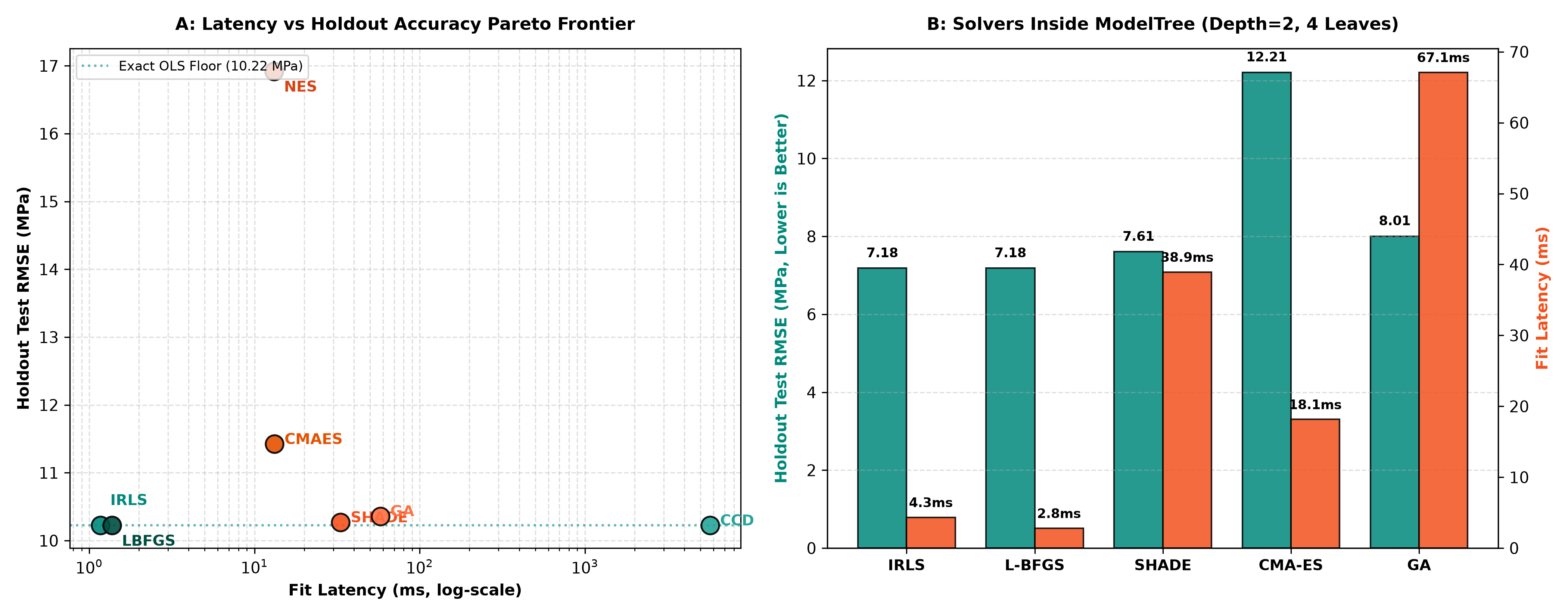
Key Observations:
- Analytical & Quasi-Newton Supremacy on Convex Surfaces:
irls(1.17 ms) andlbfgs(1.37 ms) define the Pareto frontier for smooth convex losses. Both reach identical test RMSE (10.224 MPa) at microsecond speed. - Derivative-Free Precision with SHADE:
shadeachieves 10.269 MPa (within 0.4% of the exact analytical minimum) in only 33 ms without evaluating a single gradient or Hessian. This makes it ideal for non-differentiable penalties, multi-objective fitness, or discontinuous loss landscapes. - Tree-Decoupled Leaf Performance (
max_depth=2, 4 Leaves): When deployed inside a partitioned model tree: irls: 4.34 ms total fit time \(\to\) 7.183 MPa RMSE (\(R^2 = 0.818\)).lbfgs: 2.80 ms total fit time \(\to\) 7.183 MPa RMSE (\(R^2 = 0.818\)).shade: 38.94 ms total fit time \(\to\) 7.606 MPa RMSE (\(R^2 = 0.796\)).
5. Production Recommendations
When to Select Each Solver
- Use
irlsfor standard linear ridge regression (leaf="linear") on Gaussian continuous targets. It uses Rust'sfaerdense Cholesky solver with minimal overhead. - Use
lbfgsfor GLMs (leaf_family="binomial","poisson","gamma","tweedie","tobit"). - Use
ccdwhen sparse leaves are mandatory (\(L_1 > 0\)) to eliminate irrelevant features inside leaf equations. - Use
shadewhen fitting custom non-smooth losses, quantile objectives with heavy outliers, or discontinuous simulation simulators.
References
- Nocedal, J., & Wright, S. J. (2006). Numerical Optimization. Springer.
- Tanabe, R., & Fukunaga, A. S. (2014). "Improving the search performance of SHADE using linear population size reduction." IEEE CEC, 1658-1665.
- Hansen, N. (2016). "The CMA evolution strategy: A tutorial." arXiv preprint arXiv:1604.00772.