Decision trees for credit scoring: from raw inputs to an auditable review queue
A reviewer needs to know two things about a credit score. What did the model use for this applicant, and how often does the same decision go wrong on comparable applicants? A shallow decision tree makes the first question easier to investigate. An independent test set answers part of the second.
We will estimate two-year financial distress and select a queue threshold using historical data. By the end, you will have a named tree, a confusion matrix, and a probability diagnostic. The queue is an analytical exercise. A lending policy needs separate review and evidence.
What data do you need for a credit decision tree?
Use the 150,000 labeled rows in Give Me Some Credit on OpenML. Save its Parquet file to datasets/GiveMeSomeCredit.parquet. Clone the repo, run uv sync, then run the Python code below from the root. It needs pandas and mltreelib. The full script also uses matplotlib.
The outcome is FinancialDistressNextTwoYears. Predictors include revolving utilization, delinquency counts, monthly income and number of dependents. Preserve missing income and dependent counts. Use a fixed random subset here and reserve separate observations for choosing the threshold and measuring the final results. Where application dates and repeated customers are available, split by date and entity instead.
Fit the model and choose a review threshold
from statistics import mean

from examples.real_tree_studies import load, rows
from mltreelib import Metrics, ModelTree

df = load("GiveMeSomeCredit", 46929).sample(frac=1, random_state=2026).iloc[:12000]
target = "FinancialDistressNextTwoYears"
features = df.columns.drop(target).tolist()
train, val, test = df.iloc[:8000], df.iloc[8000:10000], df.iloc[10000:]

def labels(part):
    return (part[target] == "Yes").astype(int).tolist()

tree = ModelTree(leaf="mean", leaf_family="binomial", gain="deviance",
                 max_depth=3, min_rows=100, prune="none")
tree.fit(rows(train, features), labels(train), col_names=features,
         dtypes=["numeric"] * len(features))
val_scores = tree.predict_proba(rows(val, features))

def review_cost(cutoff):
    return sum(5 if y and p < cutoff else 1 if not y and p >= cutoff else 0
               for y, p in zip(labels(val), val_scores))

cutoff = min([.02, .05, .10, .20, .40, 1.01], key=review_cost)
y = labels(test)
score = tree.predict_proba(rows(test, features))
alert = [int(p >= cutoff) for p in score]
metrics = Metrics()
print("threshold", cutoff, "confusion", metrics.classification(y, alert)["confusion"])
print("Brier tree / baseline", metrics.brier_score(y, score),
      metrics.brier_score(y, [mean(labels(train))] * len(test)))
print("one split", tree.splits()[0])
print("support", [leaf["n"] for leaf in tree.leaves()])
Five units for a missed case and one for a false alert are illustrative. Pick costs with your reviewers. The threshold lives outside the tree fit. If the review desk has a fixed number of slots, test a rank budget as a separate policy.
What do the results say?
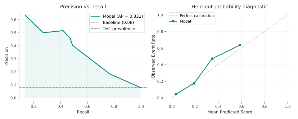
The validation threshold was 0.20. It flagged 159 of 2,000 test rows. Of the 155 observed distress events, 73 were flagged and 82 were missed. The remaining 86 alerts were false positives.
| Test metric | Tree | Reference |
|---|---|---|
| Average precision | 0.3310 | 0.0775 event prevalence |
| Brier score | 0.0577 | 0.0717 constant training rate |
The root uses revolving utilization. A later split uses the count of payments 60 to 89 days past due. The training sample contains 1,616 missing income values and 222 missing dependent counts.
Rows in the confusion matrix are observed outcomes. Columns are queue decisions. The upper-right cell counts false alerts. The lower-left cell counts missed distress events. Check both before deciding whether the queue fits the review team's capacity.
The precision–recall curve shows how the queue changes as the cutoff moves. The probability plot compares average scores and observed event rates. A useful ranking can coexist with poor probabilities. The package supplies diagnostics. Fitting a post-hoc probability calibrator is on the roadmap.
What can a tree path explain?
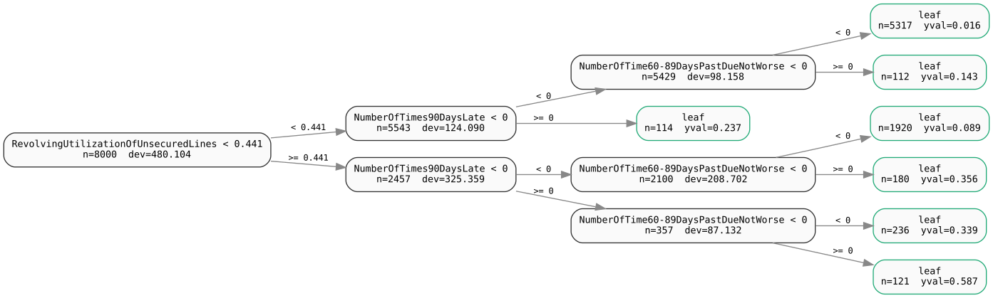
Use the diagram to read the structure. Check boundary routing before transcribing the displayed conditions.
A named split gives a condition, and the leaf stores the sample support and fitted score. Inspect the root and leaf counts before reading individual examples. To see the whole route structure, save tree.to_dot() and render it with Graphviz. Review the missing direction for any split that can encounter absent data. A displayed categorical code also needs a mapping back to its label.
The path explains the model's calculation. Credit decisions also require checking whether the variables, thresholds and outcome are appropriate. Analyze errors and review rates across applicable groups. If policy requires monotonicity, perturb the feature across split thresholds and repeat with missingness and real combinations of other features. Report any violation.
Reproduce the report
Next, compare against the same baseline on an out-of-time sample and record how much the threshold and review volume move. See the classification pathway and Brier's probability scoring paper.